Hyperbolic and Non-Euclidean Geometric Learning in the Era of LLM

Events and News!

• 📄October 1, 2026 · A Survey of Non-Euclidean Geometric Learning from Hyperbolic to Mixed-Curvature Spaces 🔥
• 📄ICML 2026 · HypRAG: Hyperbolic Dense Retrieval for Retrieval Augmented Generation (PDF)
• NeurIPS 2025 HELM: Hyperbolic Large Language Models via Mixture-of-Curvature Experts - GitHub
• 📝NeurIPS 2025 Hyperbolic Fine-tuning for Large Language Models (HypLoRA)
• 🎓KDD 2026 Hyperbolic Learning Tutorial
• 🎤KDD 2026 Geometric Learning Workshop
• 🎤NeurIPS 2025 NEGEL Workshop
• 🎓AAAI 2026 Hyperbolic FM Tutorial
• 🎓KDD 2025 Hyperbolic FM Tutorial
• 🎤WWW 2025 NEGEL Workshop
• 🎓KDD 2023 Tutorial
• Slack channel for more discussions and tracking updates!
• ⭐Awesome Hyperbolic Representation and Deep Learning Repository

Introduction

The geometry of a representation space determines how a model expresses similarity, hierarchy, and relationships. Euclidean vectors are a useful default, but their geometry may not match the structure we want to preserve. Hyperbolic space provides room for branching hierarchies; spherical space offers a compact setting for directional representations; mixed-curvature spaces combine several geometries when the data contain different kinds of structure.

In the era of large language models, these choices matter at several stages: learning token representations, building attention layers, adapting pretrained models, and organizing external knowledge for retrieval. Hyperbolic learning is one way to introduce a structural inductive bias. Its value depends on the data, the learning objective, and the computational budget, so comparisons with strong Euclidean baselines remain essential.

This page connects the geometry to the operations used in neural networks, Transformers, and foundation models. For a broader treatment of spherical and mixed-curvature learning, see our survey; the paper collection organizes research by methods, applications, and task settings.

Figure 1 · Choosing a geometry. Triangle angles sum to less than, equal to, or greater than $\pi$ in negative, zero, or positive constant curvature, respectively. A product space represents different geometric components together. The signed-curvature symbol $c$ in the figure corresponds to $\kappa$ below. For more details, please check the survey.

1. Hyperbolic Geometry

Hyperbolic space is a complete, simply connected space of constant negative sectional curvature. Its shortest paths, called geodesics, generalize straight lines. Unlike Euclidean space, its available volume grows exponentially with geodesic radius, making it a useful setting for representing branching structure.

Notation used below. $\kappa$ denotes signed sectional curvature, with $\kappa<0$ for hyperbolic space. $\lVert\cdot\rVert$ is the Euclidean norm, and $g^E=I_n$ is the Euclidean metric. Formulas for a unit Poincaré ball use $\kappa=-1$; other negative curvatures change the coordinate radius and distance scale.

1.1 Key Properties of Hyperbolic Space

Exponential area growth. In the hyperbolic plane, the area of a geodesic disk of radius $r$ is

$$A_\kappa(r)=\frac{2\pi}{-\kappa}\left[\cosh\!\left(\sqrt{-\kappa}\,r\right)-1\right].$$

For $\kappa=-1$, this grows exponentially for large $r$, while a Euclidean disk has area $\pi r^2$. The comparison concerns geodesic radius, rather than the apparent radius in a drawing. Higher-dimensional hyperbolic spaces also exhibit exponential volume growth.

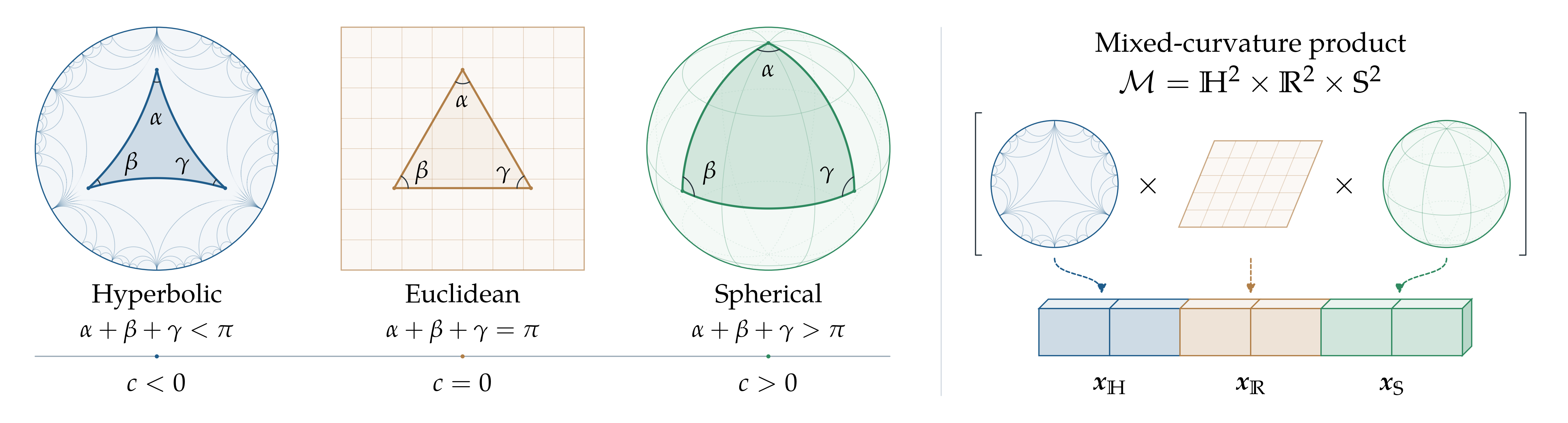
Triangle angle deficit. For a geodesic triangle in constant curvature $\kappa<0$, with angles $\alpha,\beta,\gamma$, the area is $(\pi-\alpha-\beta-\gamma)/(-\kappa)$. The angle sum is smaller than $\pi$, as illustrated in Figure 1.

An infinite space inside bounded coordinates. In the unit Poincaré ball, a point with coordinate norm $\rho=\lVert\mathbf{x}\rVert<1$ has radial distance

$$d_{\mathbb{B}}(\mathbf{0},\mathbf{x})=2\operatorname{artanh}(\rho)=\log\!\frac{1+\rho}{1-\rho}.$$

Every interior point is at a finite distance from the origin. The distance tends to infinity only as $\rho\to1$. Small coordinate differences near the boundary can therefore correspond to large geometric distances. These formulas follow the standard Poincaré model.

More room for branching structure

Geodesic radius r:

3.00

Hyperbolic disk area:

Euclidean disk area:

A finite disk represents infinite distance

Poincaré norm ρ:

0.800

Hyperbolic distance:

Euclidean distance:

The boundary ρ = 1 is excluded; hyperbolic distance tends to infinity.

Hover over a plot, drag the slider, or press Play to explore. Sliders also support arrow keys.

Figure 2 · Geometry behind the intuition. Left: disk areas at the same geodesic radius. Right: hyperbolic and Euclidean distances from the origin at the same coordinate norm $\rho$, with Euclidean distance $d_E(0,\mathbf{x})=\rho$. Red denotes hyperbolic geometry; black denotes Euclidean geometry. Hyperbolic values follow the equations above at $\kappa=-1$; these are mathematical curves, rather than experimental results.

1.2 Why Hyperbolic Geometry for AI?

A regular tree with branching factor $b>1$ has $b^d$ nodes at depth $d$. Hyperbolic volume growth offers a geometric way to accommodate that expansion. Learned embeddings can place general concepts closer to a chosen origin and more specific concepts farther out, while using directions to separate branches. This arrangement must be encouraged by the data and objective; curvature alone does not assign semantic meaning to radius.

Taxonomies, knowledge graphs, and some language or visual representations provide useful test cases. Poincaré embeddings showed that low-dimensional hyperbolic representations can perform well on hierarchical data. A power-law degree distribution or a small measured graph hyperbolicity can motivate an experiment, but neither establishes that hyperbolic geometry will outperform Euclidean geometry on every downstream task.

2. Hyperbolic Models

The Poincaré ball, Lorentz hyperboloid, Klein ball, and upper half-space describe the same hyperbolic geometry at a fixed curvature. Their coordinates and computational operations differ. Choosing a model changes how the space is represented, rather than its intrinsic distances.

2.1 Poincaré Ball Model

For signed curvature $\kappa<0$, the coordinate domain and metric are

$$\mathbb{B}_\kappa^n=\left\{\mathbf{x}\in\mathbb{R}^n:\lVert\mathbf{x}\rVert<\frac{1}{\sqrt{-\kappa}}\right\},\qquad g_{\mathbf{x}}^{\mathbb{B}}=\left(\frac{2}{1+\kappa\lVert\mathbf{x}\rVert^2}\right)^2g^E.$$

The metric is conformal: angles between tangent vectors agree with their Euclidean-coordinate angles. In two dimensions, geodesics are diameters or circular arcs orthogonal to the boundary. The distance between two points is

$$d_{\mathbb{B},\kappa}(\mathbf{x},\mathbf{y})=\frac{1}{\sqrt{-\kappa}}\operatorname{arcosh}\!\left(1-\frac{2\kappa\lVert\mathbf{x}-\mathbf{y}\rVert^2}{(1+\kappa\lVert\mathbf{x}\rVert^2)(1+\kappa\lVert\mathbf{y}\rVert^2)}\right).$$

At $\kappa=-1$, the radius is one and the metric reduces to $\left(2/(1-\lVert\mathbf{x}\rVert^2)\right)^2g^E$. The bounded picture is convenient for visualization, but computations near its boundary require care.

2.2 Lorentz (Hyperboloid) Model

For $\mathbf{x},\mathbf{y}\in\mathbb{R}^{n+1}$, define the Lorentz inner product by $\langle\mathbf{x},\mathbf{y}\rangle_{\mathcal{L}}=-x_0y_0+\sum_{i=1}^n x_iy_i$. The hyperbolic space is the upper sheet

$$\mathbb{H}_\kappa^n=\left\{\mathbf{x}\in\mathbb{R}^{n+1}:\langle\mathbf{x},\mathbf{x}\rangle_{\mathcal{L}}=\frac{1}{\kappa},\quad x_0>0\right\}.$$

The ambient inner product is indefinite, but its restriction to a tangent space gives a positive-definite Riemannian metric. The geodesic distance is

$$d_{\mathbb{H},\kappa}(\mathbf{x},\mathbf{y})=\frac{1}{\sqrt{-\kappa}}\operatorname{arcosh}\!\left(\kappa\langle\mathbf{x},\mathbf{y}\rangle_{\mathcal{L}}\right).$$

For the same point, the argument of $\operatorname{arcosh}$ is one and the distance is zero. At $\kappa=-1$, the formulas become $\langle\mathbf{x},\mathbf{x}\rangle_{\mathcal{L}}=-1$ and $d=\operatorname{arcosh}(-\langle\mathbf{x},\mathbf{y}\rangle_{\mathcal{L}})$, matching the Lorentz embedding formulation. Lorentz coordinates support efficient geometric operations, but large coordinates can still cause cancellation and precision problems.

2.3 Klein Model

The Klein model uses a ball of radius $1/\sqrt{-\kappa}$ in which geodesics appear as straight chords. It is useful for geometric constructions and some aggregation rules. Unlike the Poincaré ball, it does not preserve angles in its coordinate drawing.

2.4 Poincaré Half-Plane Model

The two-dimensional half-plane generalizes to the upper half-space $\mathbb{U}^n={\mathbf{x}\in\mathbb{R}^n:x_n>0}$. For curvature $\kappa<0$, its metric is $g_{\mathbf{x}}^{\mathbb{U}}=g^E/(-\kappa x_n^2)$. Geodesics are vertical lines or circle arcs meeting the boundary orthogonally. At $\kappa=-1$, this is the familiar metric $g^E/x_n^2$.

2.5 Inter-Model Mappings

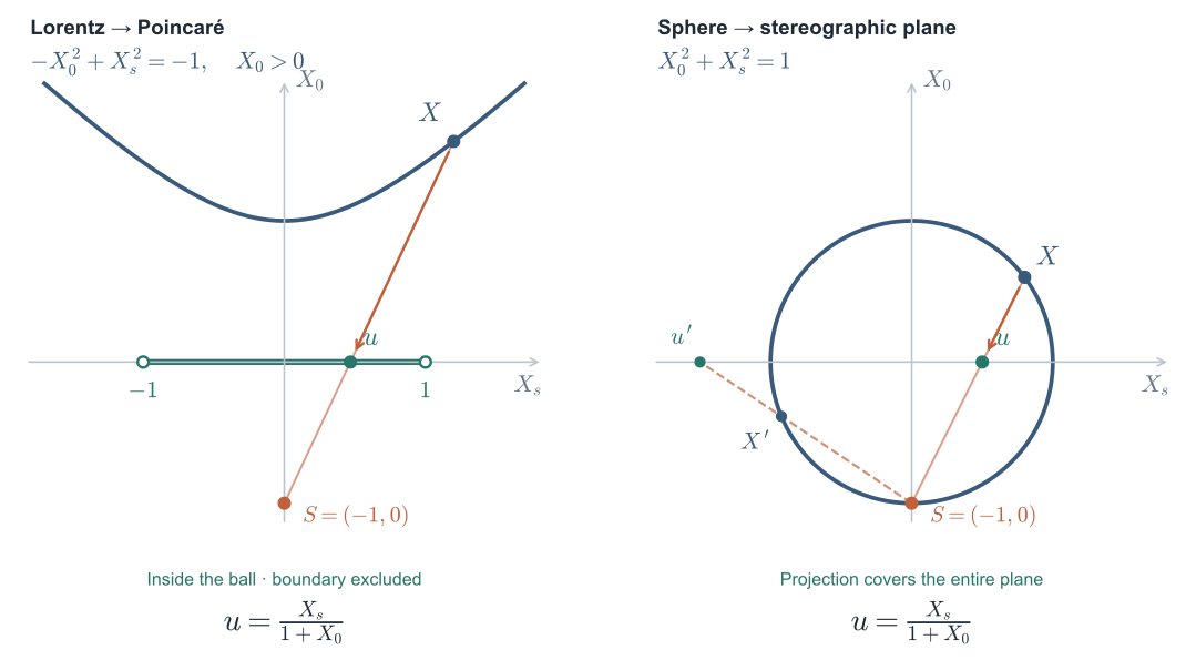
At unit curvature $\kappa=-1$, a Lorentz point $\mathbf{X}=(X_0,\mathbf{X}_s)$ maps to the Poincaré point $\mathbf{u}=\mathbf{X}_s/(X_0+1)$. The inverse map is

$$\mathbf{X}=\left(\frac{1+\lVert\mathbf{u}\rVert^2}{1-\lVert\mathbf{u}\rVert^2},\frac{2\mathbf{u}}{1-\lVert\mathbf{u}\rVert^2}\right).$$

These maps preserve intrinsic distances. One can compute in Lorentz coordinates and visualize the same points in the Poincaré ball. Neither coordinate model is universally more numerically stable; the operation, precision, and distance range matter. See the numerical stability analysis.

Figure 3 · From manifold points to coordinates. Cross-sections of the projections at unit curvature. Left: the upper hyperboloid maps inside the Poincaré ball. Right: the sphere, excluding its south pole, maps to an unbounded plane. Blue points $X$ project to green coordinates $u$ along rays from $S$; higher-dimensional models use the same construction. Click to enlarge. For more details, please check the survey.

3. Hyperbolic Neural Networks

Once representations live on a manifold, layers must respect its geometry. A practical design specifies where features live, how transformations and aggregation act, and how outputs remain valid points. Euclidean parameters can still be used to construct manifold-valued representations.

3.1 Hyperbolic Embeddings

An embedding assigns each entity a point and trains distances or similarity scores to reflect the desired relationships. Poincaré embeddings established this approach for hierarchies; Lorentz embeddings offered an alternative coordinate system for optimization. Low dimensionality and a meaningful radial organization are possible outcomes of training, rather than properties guaranteed for every dataset.

3.2 Hyperbolic Neural Layers

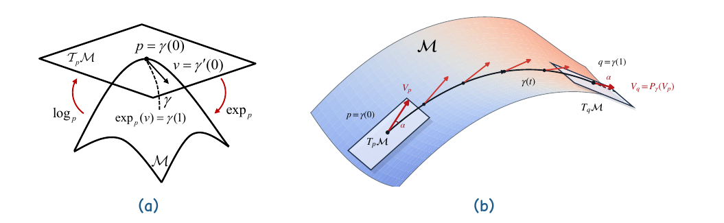
Tangent-space layers use $\log_{\mathbf{p}}$ to map a manifold point to a vector at a reference point $\mathbf{p}$, apply a Euclidean operation, then return with $\exp_{\mathbf{p}}$. These maps are exact on hyperbolic space; the resulting Euclidean operation is a design choice and does not automatically preserve hyperbolic distances.

Möbius layers define ball operations that keep outputs in the domain. A bias-free transformation can be written as $\mathbf{M}\otimes_\kappa\mathbf{x}=\exp_{\mathbf{0}}^\kappa(\mathbf{M}\log_{\mathbf{0}}^\kappa(\mathbf{x}))$, followed by a Möbius bias addition. This connects gyrovector operations to neural layers in Hyperbolic Neural Networks.

Direct Lorentz layers construct a valid hyperboloid point from learned spatial coordinates. For example, spatial output $\mathbf{z}$ can be completed with time coordinate $x_0=\sqrt{\lVert\mathbf{z}\rVert^2-1/\kappa}$. This enforces the manifold constraint, although it does not by itself make the layer distance-preserving.

Figure 4 · The operations behind geometric layers. The exponential map follows a geodesic from a tangent vector to a manifold point; the logarithmic map reverses that construction. Parallel transport moves a tangent vector between tangent spaces while preserving its norm. For more details, please check the survey.

3.3 Key Architectures

• HNN and HNN++: building blocks for hyperbolic feed-forward, recurrent, and attention-based networks.
• HGCN and HGNN: geometric feature transformations and neighborhood aggregation for graphs.
• Fully Hyperbolic Neural Networks: Lorentz-valued layers and attention without repeatedly using a common tangent space.
• $\kappa$-GCN: graph learning in a shared stereographic formulation spanning negative, zero, and positive curvature.

3.4 Hyperbolic Activation Functions

A common activation applies $\sigma$ to tangent coordinates and maps the result back: $\sigma_{\mathcal{M}}(\mathbf{x})=\exp_{\mathbf{p}}(\sigma(\log_{\mathbf{p}}(\mathbf{x})))$. Other constructions act on Lorentz spatial coordinates and rebuild the time coordinate. Applying an ordinary coordinate-wise activation directly to a manifold point generally fails to preserve its constraint.

3.5 Optimization in Hyperbolic Space

For a parameter $\mathbf{x}$ constrained to the manifold, the Riemannian gradient belongs to its tangent space. A Riemannian SGD step is

$$\mathbf{x}_{t+1}=\exp_{\mathbf{x}_t}\!\left(-\eta_t\operatorname{grad}f(\mathbf{x}_t)\right).$$

Here $\eta_t>0$ is the learning rate. Implementations may use a suitable retraction instead of the exponential map. In the Poincaré model, the Riemannian gradient is $(\lambda_{\mathbf{x}}^\kappa)^{-2}\nabla f(\mathbf{x})$, where $\lambda_{\mathbf{x}}^\kappa=2/(1+\kappa\lVert\mathbf{x}\rVert^2)$. Adaptive methods must also account for tangent-space geometry; see Riemannian Adaptive Optimization Methods.

4. Hyperbolic Transformers

A Transformer combines projections, attention, value aggregation, residual connections, normalization, and position information. A hyperbolic version must define each component consistently. Mapping an ordinary Transformer’s output embeddings to a manifold is useful, but it is a different architectural choice from performing its internal layers in hyperbolic space.

4.1 Hyperbolic Attention Mechanisms

Standard attention produces an output $\operatorname{softmax}(\mathbf{Q}\mathbf{K}^{\mathsf{T}}/\sqrt{d_k})\mathbf{V}$. In a distance-based geometric variant, queries and keys are manifold points and the attention weights can be

$$\alpha_{ij}=\frac{\exp\!\left[-\beta d_{\mathbb{H},\kappa}(\mathbf{q}_i,\mathbf{k}_j)^2\right]}{\sum_{\ell=1}^{N}\exp\!\left[-\beta d_{\mathbb{H},\kappa}(\mathbf{q}_i,\mathbf{k}_\ell)^2\right]},\qquad\beta>0.$$

The denominator normalizes over keys for a fixed query; $\beta$ is an inverse temperature. A complete layer must also specify how the values are combined. An ordinary weighted coordinate sum generally leaves the manifold, so geometric means, normalized Lorentz centroids, or tangent-space aggregation are used. This distinction appears explicitly in fully hyperbolic attention.

Geodesic proximity depends on both radius and direction. Two tokens at the same radius can belong to different branches and be far apart; radial depth alone does not determine attention. Other designs use Lorentz inner products or tangent-space dot products, and efficient variants need not compute every pairwise distance.

4.2 Multi-Resolution Processing

When the objective learns a hierarchy, radius can encode depth and direction can distinguish branches. Attention can then connect general and specific representations. Such a structure must be measured in the trained embeddings; operating in hyperbolic space does not automatically provide a multi-resolution decomposition.

4.3 Hyperbolic Position Encodings

Sequence position and semantic hierarchy serve different roles. Positional mechanisms must respect the chosen geometric operations while retaining useful relative-position information. HELM develops hyperbolic rotary positional encoding, along with geometry-aware normalization, for this purpose.

4.4 Notable Hyperbolic Transformer Models

The names below follow the papers. Model names link to the papers, and venues link to their publication records. Years refer to conference publication rather than the first preprint.

Name used in the paper	Key characteristics	Venue	Year
HELM-MiCE	Mixture-of-Curvature Experts with distinct learned negative curvatures; hyperbolic Multi-Head Latent Attention reduces the KV cache. Shares HELM's positional and normalization modules.	NeurIPS	2025
HELM-D	Dense, fully hyperbolic decoder-only language model with hyperbolic rotary positions and RMS normalization; pretrained at billion-parameter scale.	NeurIPS	2025
Hypformer	Lorentz-space Transformer blocks for projections, normalization, activation, and dropout; linear self-attention supports large graphs and long sequences.	KDD	2024
HyboNet	Direct Lorentz linear layers and attention using geometric centroids. The framework includes a fully hyperbolic Transformer evaluated on machine translation and syntax probing.	ACL	2022
Hyperbolic Attention Networks	Hyperbolic attention weights and geometric value aggregation; other Transformer blocks remain Euclidean. An early approach evaluated on translation, graphs, and visual question answering.	ICLR	2019

Mixed-curvature product embeddings provide a related geometric foundation. They combine model spaces, but are not themselves a Transformer architecture.

5. Hyperbolic Foundation Models

Geometry can enter a foundation-model pipeline through pretraining, parameter-efficient adaptation, embedding heads, or external retrieval. These routes change different components and should be evaluated accordingly. A geometric retrieval head, for example, does not make the underlying language model fully hyperbolic.

5.1 Hyperbolic Large Language Models

HypLoRA applies low-rank adaptation in hyperbolic space. Its paper studies token geometry and reports improvements on arithmetic and commonsense reasoning benchmarks. This provides evidence for a particular adaptation method and experimental setting, rather than a guarantee for every language task.

HELM studies fully hyperbolic pretraining at billion-parameter scale. Its dense model and Mixture-of-Curvature Experts variant use hyperbolic operations throughout the architecture. The experts in HELM-MiCE learn different negative curvatures; this should not be described as a mixture of hyperbolic, Euclidean, and spherical experts.

Geometric retrieval and memory apply structured representations outside the parameterized model. Their evaluation should separate retrieval quality, generated-answer quality, update behavior, and computational cost.

5.2 Hyperbolic Vision Foundation Models

Hyperbolic Image Embeddings explores visual representations in curved space. Hyperbolic Vision Transformers uses a vision Transformer encoder whose output embeddings are mapped to hyperbolic space for metric learning; it does not establish that every internal attention or positional operation is hyperbolic.

MERU learns image-text representations in a shared hyperbolic space. It is a concrete example of geometric multimodal representation learning, rather than a claim that standard CLIP already uses hyperbolic geometry.

5.3 Hyperbolic Multi-Modal Models

Image and text representations can be aligned through a shared geometric space and an appropriate learning objective. Hierarchical entailment constraints can distinguish a general description from a more specific image or phrase. This goes beyond making paired representations close: it asks the geometry to encode relationships between levels of specificity, as explored in MERU.

Where modalities contain heterogeneous structure, a product of hyperbolic, Euclidean, and spherical factors is another option. The choice of factors, dimensions, and curvature remains part of the model design and must be validated.

5.4 Key Advantages

The main opportunity is to represent a task’s structure with an appropriate geometric bias. Potential benefits include lower-dimensional hierarchical embeddings, explicit relations between general and specific concepts, and better retrieval or adaptation on suitable data. These benefits are conditional: fewer embedding dimensions do not automatically imply lower end-to-end latency, stronger reasoning, or better scaling. Performance and cost should be measured together.

6. Challenges and Opportunities

Numerical precision. Boundary effects in ball coordinates and cancellation in large Lorentz coordinates can both cause errors. Stable formulas, controlled radii, and suitable precision are necessary. Geometry-sensitive operations may need higher precision even when the rest of a network uses mixed precision. The numerical stability study explains why neither model is a universal solution.

Optimization and curvature. Gradient scaling, initialization, transport, and manifold constraints affect training. Learnable curvature adds flexibility, but can interact with representation scale and numerical conditioning. Parameters living in Euclidean space and points constrained to a manifold also need different optimization treatment.

Scaling and integration. Billion-parameter hyperbolic language models have already been explored in HELM. Open questions include reliable training at larger scales, efficient kernels, KV-cache behavior, and comparisons at matched compute. Selective geometric adapters or retrieval modules offer another practical route.

Evaluation. Match parameter counts, training data, optimization effort, and compute budgets when possible. Report task performance alongside numerical failures, distortion, retrieval behavior, memory usage, and latency. Ablations should distinguish the effect of curvature from the effect of a changed architecture or objective.

Broader geometric structure. Product spaces allow heterogeneous relationships to be represented together. With a standard Riemannian product metric, the product space and its squared distance are

$$\mathcal{M}=\mathcal{M}_1\times\cdots\times\mathcal{M}_m,$$ $$d_{\mathcal{M}}(\mathbf{x},\mathbf{y})^2=\sum_{j=1}^{m}d_{\mathcal{M}_j}(\mathbf{x}_j,\mathbf{y}_j)^2.$$

Choosing suitable factors and testing whether their structure is useful remain central questions for mixed-curvature learning.

7. Conclusion

Hyperbolic and non-Euclidean learning make representation geometry an explicit design choice. The key is to connect a geometric property to a modeling need, define the corresponding operations correctly, and test the resulting system against appropriate alternatives. Hierarchical embeddings, geometric Transformers, adaptation, and retrieval provide concrete settings in which to make that connection.

Continue with the survey for mathematical foundations and a broader research overview, the collection for papers organized by topic, or the events page for tutorials and workshops.

Contributors

Menglin Yang, Neil He, Hiren Madhu, Ngoc Bui, Ali Maatouk, Rishabh Anand, Yifei Zhang, Jialin Chen, Jiahong Liu, Bo Xiong, Min Zhou, Irwin King, Melanie Weber, Rex Ying

Invited Speakers: Philip S. Yu, Shirui Pan, Min Zhou, Pascal Mettes, Smita Krishnaswamy

References

1. Adcock, A. B., Sullivan, B. D., & Mahoney, M. W. (2013). Tree-like structure in large social and information networks. ICDM.
2. Bachmann, G., Bécigneul, G., & Ganea, O. (2020). Constant Curvature Graph Convolutional Networks. ICML. arXiv:1911.05076
3. Bécigneul, G., & Ganea, O. (2019). Riemannian Adaptive Optimization Methods. ICLR. arXiv:1810.00760
4. Bonnabel, S. (2013). Stochastic Gradient Descent on Riemannian Manifolds. IEEE Transactions on Automatic Control, 58(9).
5. Chami, I., Ying, R., Ré, C., & Leskovec, J. (2019). Hyperbolic Graph Convolutional Neural Networks. NeurIPS. arXiv:1910.12933
6. Chen, W., Han, X., Lin, Y., Zhao, H., Liu, Z., Li, P., Sun, M., & Zhou, J. (2022). Fully Hyperbolic Neural Networks. ACL. arXiv:2105.14686
7. Desai, K., Nickel, M., Rajpurohit, T., Johnson, J., & Vedantam, R. (2023). Hyperbolic Image-Text Representations (MERU). ICML. arXiv:2304.09172
8. Ermolov, A., Mirvakhabova, L., Khrulkov, V., Sebe, N., & Oseledets, I. (2022). Hyperbolic Vision Transformers: Combining Improvements in Metric Learning. CVPR. arXiv:2203.10833
9. Ganea, O., Bécigneul, G., & Hofmann, T. (2018). Hyperbolic Neural Networks. NeurIPS. arXiv:1805.09112
10. Gromov, M. (1987). Hyperbolic Groups. In Essays in Group Theory, MSRI Publ., Springer.
11. Gu, A., Sala, F., Gunel, B., & Ré, C. (2019). Learning Mixed-Curvature Representations in Product Spaces. ICLR. OpenReview
12. He, N., Yang, M., et al. (2025). HELM: Hyperbolic Large Language Models via Mixture-of-Curvature Experts. NeurIPS. arXiv:2505.24722
13. Khrulkov, V., Mirvakhabova, L., Ustinova, E., Oseledets, I., & Lempitsky, V. (2020). Hyperbolic Image Embeddings. CVPR. arXiv:1904.02239
14. Liu, Q., Nickel, M., & Kiela, D. (2019). Hyperbolic Graph Neural Networks. NeurIPS. arXiv:1910.12892
15. Nickel, M., & Kiela, D. (2017). Poincaré Embeddings for Learning Hierarchical Representations. NeurIPS. arXiv:1705.08039
16. Nickel, M., & Kiela, D. (2018). Learning Continuous Hierarchies in the Lorentz Model of Hyperbolic Geometry. ICML. arXiv:1806.03417
17. Sarkar, R. (2011). Low Distortion Delaunay Embedding of Trees in Hyperbolic Plane. Graph Drawing.
18. Shimizu, R., Mukuta, Y., & Harada, T. (2021). Hyperbolic Neural Networks++. ICLR. arXiv:2006.08210
19. Ungar, A. A. (2008). Analytic Hyperbolic Geometry and Albert Einstein's Special Theory of Relativity. World Scientific.
20. Yang, M., Verma, H., Zhang, D. C., Liu, J., King, I., & Ying, R. (2024). Hypformer: Exploring Efficient Transformer Fully in Hyperbolic Space. KDD. arXiv:2407.01290
21. Yang, M. et al. (2025). Hyperbolic Fine-tuning for Large Language Models (HypLoRA). NeurIPS.
22. Mishne, G., Wan, Z., Wang, Y., & Yang, S. (2023). The Numerical Stability of Hyperbolic Representation Learning. ICML. arXiv:2211.00181